matlab求解最优化函数

linprog
intlinprog
quadprog
fminbnd
fmincon
fseminf
fminunc
fminmax

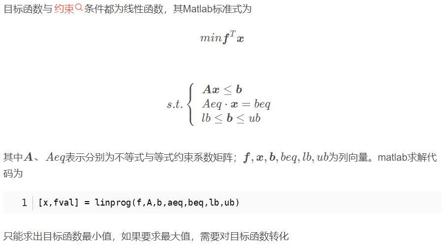
线性规划

一般形式

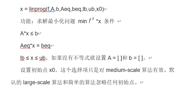
加x0的形式

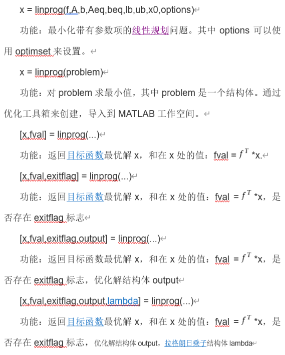
其他形式

有约束

实例1

题目

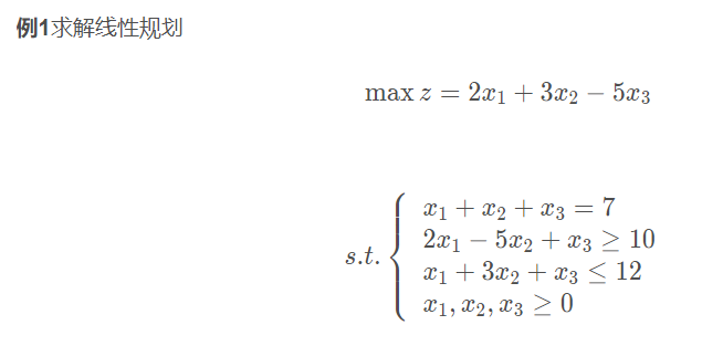
代码


% 规划问题与matlab
%---------------------线性规划------------------
% 线性规划求解
% 例1
clc;clear;close all;
f = [-2; -3; 5]; %matlab的向量为列向量
A = [-2, 5, -1; 1, 3, 1]; %系数矩阵
b = [-10, 12]; % 常数项
Aeq = [1, 1, 1]; % 等式矩阵
beq = 7; %等式对应的常数向量
l = zeros(3, 1);
u = [];
[x,y] = linprog(f, A, b, Aeq, beq, l, u) %zeros(3,1)解的下限都为正

实例2

题目

代码


xxxxxxxxxx
clear;
f = [3;-1;-1];
A = [1,-2,1;4,-1,-2];
b = [11,-3];
Aeq = [-2,0,1];
beq = 1;
l = zeros(3, 1);
u = [];
[x, y] = linprog(-f, A, b, Aeq, beq, l, u)

实例2

题目

代码


x
clear;clc;close all;
hold on;
b = [11,-3];
aeq = [-2,0,1];
beq = 1;
f = [3;-1;-1];

for i = 0 : 0.05 : 10
    a = [i*1,-2,1;4,-1,-2];
    [x,y] = linprog(-f,a,b,aeq,beq,zeros(3,1));
    y = -y;
    plot(i, y,"*r");
end

xlabel("参数");
ylabel("目标函数值");
hold off;

无约束

非线性规划

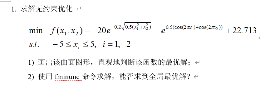
无约束

fminunc

实例1

题目

代码


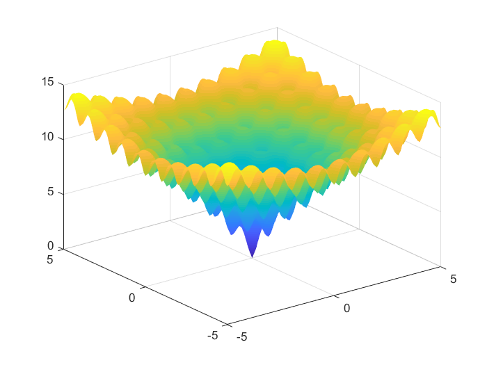
xxxxxxxxxx
clear; clc; close all;
%%
% -5 <= x, y <= 5
x = -5 : 0.1 : 5;
y = -5 : 0.1 : 5;
f = @(x) -20 * exp(-0.2 * sqrt(0.5 * (x(1).^2 + x(2).^2)))...
    - exp(0.5 * (cos(2 * pi * x(1)) + cos(2 * pi * x(2)))) + 22.713;

f1 = @(x, y) -20 * exp(-0.2 * sqrt(0.5 * (x.^2 + y.^2)))...
    - exp(0.5 * (cos(2 * pi * x) + cos(2 * pi * y))) + 22.713;
%% 画图
[X, Y] = meshgrid(x, y);
Z = f1(X, Y);

surf(X, Y, Z);
shading interp; %使surf绘制的 曲面图 表面光滑

figure
%% 数值计算
options = optimoptions('fminunc','Display','off',...
    'OutputFcn',@bananaout,'Algorithm','quasi-newton');
[x, fval, eflag, output] = fminunc(f, [0, 1], options)

效果

实例2

题目

代码


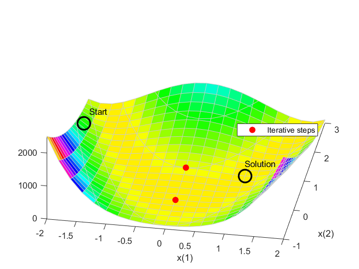
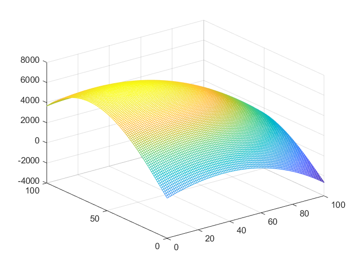
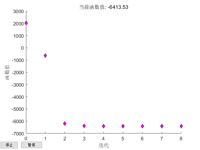
xxxxxxxxxx
clear;
clc;
close all;
%%
a = [1, 0.1; 0.2, 2];
b = [100, 280];
r = [30, 100];
landa = [0.015, 0.02];
c = [20, 30];
%% 匿名函数 元胞
for i = 1 : 1: 2
    q{i} = @(x) r(i)*exp(-landa(i) * x) + c(i);
    p{i} = @(x1, x2) b(i) - a(i, 1) * x1 - a(i, 2) * x2;
end
z = @(x1, x2) (p{1}(x1, x2) - q{1}(x1)) .* x1 + (p{2}(x1, x2) - q{2}(x2)) .* x2;
z1 = @(x) -((p{1}(x(1), x(2)) - q{1}(x(1))) .* x(1) + (p{2}(x(1), x(2)) - q{2}(x(2))) .* x(2)...
    - (x(1)<0)*10^5 - (x(2)<0)*10^5); % 无约束变成有约束（罚函数）
%% 画图
x = 0:1:100;
y = 0:1:100;
[X, Y] = meshgrid(x, y);
Z = z(X, Y);
mesh(X, Y, Z);
%% 数值计算
% options = optimoptions('fminunc','Display','off',...
%     'OutputFcn',@bananaout,'Algorithm','quasi-newton');
options=optimoptions(@fminunc,'Display','iter','PlotFcns',@optimplotfval,'Algorithm','quasi-newton');
[x, fval, eflag, output]=fminunc(z1, [100, 100], options);
% xlim([0,2]);
% ylim([0,2]);
% zlim([-5000,5000])
%axis([0,50,0,70,-10^4,0])

效果

有约束

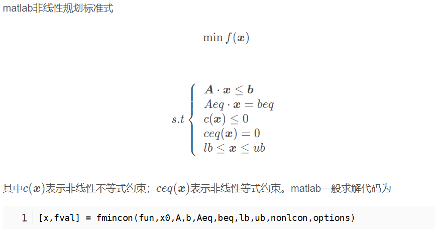
一般形式

求解过程

实例1

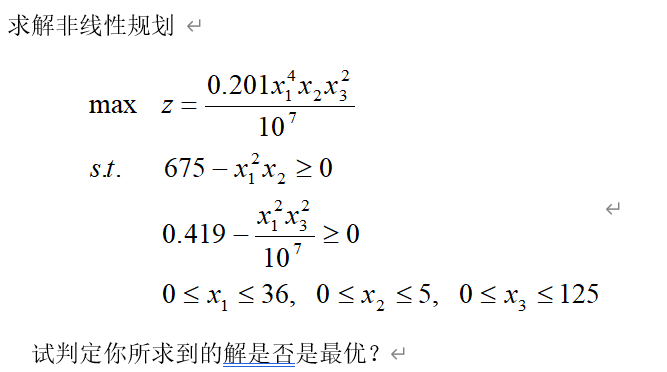
题目

代码

t_s_3_3_func函数代码


xxxxxxxxxx
function [C,Ceq]=t_s_3_3_func(x)
C(1) = x(1).^2 .* x(2) - 675;
C(2) = x(1).^2 .* x(3).^2 / 1e7 - 0.419;
Ceq = [];
end

主函数文件代码


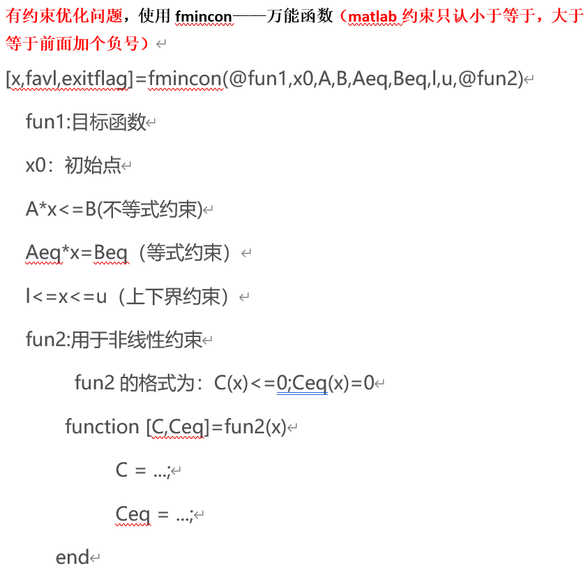
xxxxxxxxxx
%{
[x,favl,exitflag]=fmincon(@fun1,x0,A,B,Aeq,Beq,l,u,@fun2)
   fun1:目标函数
   x0：初始点
   A*x<=B(不等式约束)
   Aeq*x=Beq（等式约束）
   l<=x<=u（上下界约束）
   fun2:用于非线性约束
           fun2的格式为：C(x)<=0;Ceq(x)=0
        function [C,Ceq]=fun2(x)
               C = ...;
               Ceq = ...;
       end
%}
clear; clc; close all;
%%
fun1 = @(x) -(0.201 * x(1).^4 .* x(2) .* x(3).^2) / 1e7; %目标函数
A = [];
B = [];
l = zeros(1,3);
u = [36, 5, 125];
Aeq = [];
Beq = [];
x0 = [0, 0, 0];
%%
[x,fval,exitflag] = fmincon(fun1,x0,A,B,Aeq,Beq,l,u,@t_s_3_3_func);
x
-fval

实例2

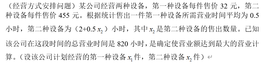
题目

代码

t_s_3_4_func函数文件代码


xxxxxxxxxx
function [C,Ceq] = t_s_3_4_func(x)
C = [];
Ceq(1) = x(1) * 0.5 + x(2) .* (2 + 0.5 * x(2)) - 820;
end

主函数文件代码


xxxxxxxxxx
clear; clc; close all;
%%
%{
t1、t2 第一、第二种设备销售的总时间
%% 模型建立
t1 + t2 = 820;
t1 = x1 * 0.5;
t2 = x2 * (2 + 0.5 * x2);

=>
x1 * 0.5 + x2 * (2 + 0.5 * x2) = 820; % 非线性约束
x1 >= 0; x2 >= 0;
max z = 32x1 + 455x2;
%}
%%
func1 = @(x) -(32 * x(1) + 455 * x(2));
l = [0, 0];
u = [];
A = [];
B = [];
Aeq = [];
Beq = [];
x0 = [0, 0];
[x,fval,exitflag]=fmincon(func1,x0,A,B,Aeq,Beq,l,u,@t_s_3_4_func);
x
-fval

整数规划

数学规划中的变量（部分或者全部）限制为整数时，称为整数规划。
若在线性规划模型中，变量限制为整数，则称为整数线性规划。

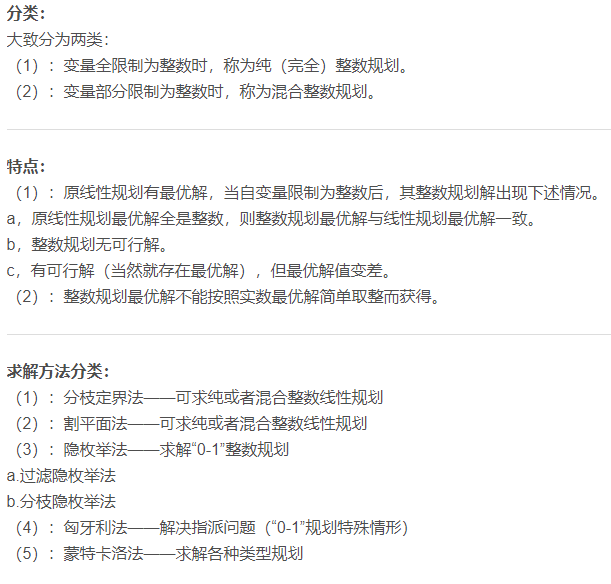
整数线性规

一般形式

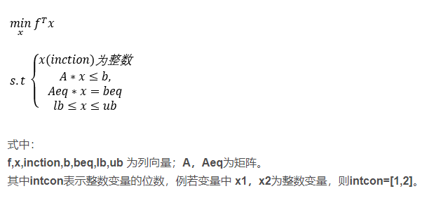
intcon向量：intcon=[1,3,5]代表x1、x3、x5为整数

注意

把变量取值限制在[0,1]就是整数规划了。。。

例题

实例1

题目

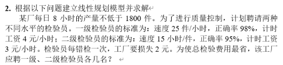
代码


x
clear; clc; close all;
%%
% x1, x2
% min z = 8*(4*x1 + 3*x2 + 2*(0.02*x1 + 0.05*x2));
% x1 >= 0, x2 >= 0
% 0.98*25*x1 + 0.95*15*x2 >= (1800/8)=225
%%
% z = @(x1, x2) 4*x1 + 3*x2 + 8*2*(0.02*x1 + 0.05*x2);
C = [32 + 16*0.02, 24 + 16 * 0.05];
A = -[0.98*25, 0.95*15];
b = -225;
Aeq = [];
beq = [];
l = [0, 0];
u = [];
intcon=[1, 2];
[x, y] = intlinprog(C, intcon, A, b, Aeq, beq, l, u)

结果